DeepLagField: Time-Varying AR Reconstruction

This tutorial demonstrates training a neural network to infer the order \(p\) and time-varying coefficients \(a(t)\) of TVAR processes:

\[x_t = \sum_{k=1}^{p} a_k(t) x_{t-k} + \varepsilon_t\]

Goals:

1. Generate synthetic TVAR data with known ground-truth coefficients

2. Train DeepLagField to jointly predict AR order and coefficient trajectories

3. Evaluate classification and regression accuracy across coefficient families

import torch
from torch.utils.data import DataLoader, TensorDataset
from sklearn.metrics import confusion_matrix, ConfusionMatrixDisplay
import numpy as np
from tqdm import tqdm
import matplotlib.pyplot as plt
import pandas as pd

from NeuralFieldManifold.models import DeepLagEmbed
from NeuralFieldManifold.generators import tvar
from NeuralFieldManifold.utils import train_loop, bench_loop
from NeuralFieldManifold.plottings import plot_history, plot_coefficients_by_p, plot_tvar_sample
from NeuralFieldManifold.generators import (
    sinusoid,
    fourier,
    quasiperiodic,
    polynomial_drift,
    logistic_transition,
    multi_sigmoid,
    gaussian_bumps,
    smooth_random,
)
from torchinfo import summary
from concurrent.futures import ProcessPoolExecutor, as_completed
import multiprocessing
from utils import pinn_processor

Coefficient Schedule Registry

Eight families control how \(a_k(t)\) evolve over time:

• sinusoid / fourier / quasiperiodic: Periodic or near-periodic oscillations

• poly_drift / logistic: Smooth trends and transitions

• multi_sigmoid / gaussian_bumps: Localized regime changes

• smooth_random: Stochastic but differentiable trajectories

# Registry of families you can benchmark
SCHEDULES = {
    "sinusoid": sinusoid,
    "fourier": fourier,
    "quasiperiodic": quasiperiodic,
    "poly_drift": polynomial_drift,
    "logistic": logistic_transition,
    "multi_sigmoid": multi_sigmoid,
    "gaussian_bumps": gaussian_bumps,
    "smooth_random": smooth_random,
}

Data Generation

Key functions:

• simulate_tvar(): Simulates TVAR with soft power clamping to prevent divergence

• generate_one_tvar_sample(): Produces a single \((x, a(t), \text{meta})\) tuple with retry logic

• generate_dataset(): Parallelized generation balanced across families and orders \(p \in \{2,...,6\}\)

def _rng(seed):
    return np.random.default_rng(seed)

def pad_to_pmax(a_time_p, p_max):
    """Pad [T, p_true] -> [T, p_max] with zeros."""
    T, p = a_time_p.shape
    out = np.zeros((T, p_max), dtype=a_time_p.dtype)
    out[:, :p] = a_time_p
    return out

def generate_one_tvar_sample(
    T=10_000,
    p_max=6,
    schedule_name="sinusoid",
    noise_std=0.3,
    seed=0,
    l1_cap=0.95,
    P0=0.5,
    W=40,
    power_control=True,
    p_true=None,  # If provided, use this p; otherwise random
    p_candidates=None,
    max_retries=10000,  # Maximum resampling attempts
):
    rng = _rng(seed)
    if p_candidates is None:
        p_candidates = np.array([2, 3, 4, 5, 6], dtype=int)
    
    # Use provided p_true or randomly select
    if p_true is None:
        p_true = int(rng.choice(p_candidates))
    else:
        p_true = int(p_true)

    # Retry loop: resample until we get a valid sample
    current_seed = seed
    for attempt in range(max_retries):
        # Use a fresh rng for coefficient schedule each attempt
        attempt_rng = _rng(current_seed)
        
        # coefficient schedule for true p
        a_tp = SCHEDULES[schedule_name](T=T, p=p_true, rng=attempt_rng)

        # simulate signal with power control (rejection-based)
        x, a_actual = simulate_tvar(
            a_tp, noise_std=noise_std, seed=current_seed+123,
            P0=P0, W=W, power_control=power_control
        )

        # If valid sample (not rejected), break out
        if x is not None:
            break
        
        # Increment seed for next attempt
        current_seed += 1
    else:
        raise RuntimeError(f"Failed to generate valid sample after {max_retries} retries for schedule '{schedule_name}', p_true={p_true}")

    # pad coeffs to p_max for consistent storage
    a_t = pad_to_pmax(a_actual.astype(np.float32), p_max)

    meta = {
        "T": T,
        "p_max": p_max,
        "p_true": p_true,
        "schedule": schedule_name,
        "noise_std": float(noise_std),
        "seed": int(current_seed),  # Record the seed that actually worked
        "l1_cap": float(l1_cap),
        "P0": float(P0),
        "W": int(W),
        "power_control": power_control,
        "p_candidates": list(p_candidates),
        "retries": attempt,  # Number of retries needed
    }
    return x, a_t, meta

def _generate_sample_worker(args):
    """
    Worker function for parallel sample generation.
    Takes a dict of arguments and returns (idx, x, a_t, meta, cid, ns).
    """
    idx = args["idx"]
    T = args["T"]
    p_max = args["p_max"]
    cname = args["cname"]
    ns = args["ns"]
    s = args["s"]
    P0 = args["P0"]
    W = args["W"]
    power_control = args["power_control"]
    p_true_val = args["p_true_val"]
    p_candidates = args["p_candidates"]
    cid = args["cid"]
    
    x, a_t, meta = generate_one_tvar_sample(
        T=T, p_max=p_max, schedule_name=cname, noise_std=ns, seed=s,
        P0=P0, W=W, power_control=power_control,
        p_true=p_true_val, p_candidates=p_candidates,
    )
    
    return idx, x, a_t, meta, cid, ns

def simulate_tvar(a_time, noise_std=0.3, seed=0, burn_in=300,
                  P0=0.5, W=40, power_control=True,
                  divergence_threshold=1e6):
    """
    Simulate a TVAR process with soft power clamping and hard rejection safety net:
        x_t = a(t)^T [x_{t-1}, ..., x_{t-p}] + eps_t

    During simulation, if window power exceeds P0, the current sample is scaled
    by clip(sqrt(P0/power), 0.8, 1.2) to gently steer power back toward the target.
    After simulation, a final hard check rejects if power still exceeds P0.
    """
    rng = _rng(seed)
    T, p = a_time.shape

    T_full = T + int(burn_in)
    x_full = np.zeros(T_full, dtype=np.float64)
    eps = rng.normal(0.0, noise_std, size=T_full)

    x_full[:p] = eps[:p]

    for t in range(p, T_full):
        tau = t - int(burn_in)
        if tau < 0:
            a_t = a_time[0]
        else:
            a_t = a_time[min(tau, T - 1)]

        lags = x_full[t-p:t][::-1]
        x_full[t] = np.dot(a_t, lags) + eps[t]

        # Early divergence check — fail fast instead of letting values blow up
        if abs(x_full[t]) > divergence_threshold:
            return None, None

        # Soft power clamping (matches the working tvar() function)
        if power_control and t >= W - 1:
            window = x_full[t - W + 1:t + 1]
            current_power = np.mean(window ** 2)
            if current_power > 0:
                s = np.clip(np.sqrt(P0 / current_power), 0.8, 1.2)
                x_full[t] *= s

    # Drop burn-in (safe cast now — divergent runs already returned None)
    x = x_full[int(burn_in):].astype(np.float32)

    # Hard rejection safety net: only check full W-sized windows
    # (matches soft clamping which only activates at t >= W-1)
    if power_control and len(x) >= W:
        x2 = x ** 2
        cumsum = np.concatenate([[0.0], np.cumsum(x2)])
        ends = np.arange(W, len(x) + 1)
        starts = ends - W
        power = (cumsum[ends] - cumsum[starts]) / W
        if np.any(power > P0):
            return None, None

    return x, a_time

def generate_dataset(
    n_per_class=10,
    classes=None,
    T=1000,
    noise_range=(0.1, 0.6),
    seed=0,
    dtype=np.float32,
    P0=0.5,
    W=40,
    power_control=True,
    p_candidates=None,
    balanced_p=True,  # If True, balance samples across p_candidates
    n_workers=None,  # Number of parallel workers (None = CPU count)
):
    
    p_max = 10
    
    if p_candidates is None:
        p_candidates = np.array([2, 3, 4, 5, 6], dtype=int)
    else:
        p_candidates = np.array(p_candidates, dtype=int)

    if classes is None:
        classes = list(SCHEDULES.keys())

    if n_workers is None:
        n_workers = multiprocessing.cpu_count()

    rng = _rng(seed)
    N = n_per_class * len(classes)

    X = np.zeros((N, T), dtype=dtype)
    A = np.zeros((N, T, p_max), dtype=dtype)
    p_true_arr = np.zeros((N,), dtype=np.int32)
    class_id = np.zeros((N,), dtype=np.int32)
    noise_std = np.zeros((N,), dtype=dtype)

    class_names = list(classes)
    
    # Precompute p assignments if balanced
    n_p = len(p_candidates)
    if balanced_p:
        n_per_p = n_per_class // n_p
        remainder = n_per_class % n_p
        # Create balanced p assignments for one class
        p_assignments = []
        for i, p in enumerate(p_candidates):
            count = n_per_p + (1 if i < remainder else 0)
            p_assignments.extend([p] * count)
    
    # Build all task arguments
    tasks = []
    idx = 0
    for cid, cname in enumerate(class_names):
        # Shuffle p assignments for this class
        if balanced_p:
            class_p_assignments = rng.permutation(p_assignments)
        
        for i in range(n_per_class):
            s = int(rng.integers(0, 2**31 - 1))
            ns = float(rng.uniform(noise_range[0], noise_range[1]))
            
            # Determine p_true
            if balanced_p:
                p_true_val = int(class_p_assignments[i])
            else:
                p_true_val = None  # Let generate_one_tvar_sample pick randomly
            
            tasks.append({
                "idx": idx,
                "T": T,
                "p_max": p_max,
                "cname": cname,
                "ns": ns,
                "s": s,
                "P0": P0,
                "W": W,
                "power_control": power_control,
                "p_true_val": p_true_val,
                "p_candidates": list(p_candidates),
                "cid": cid,
            })
            idx += 1
    
    metas = [None] * N
    
    # Parallel execution
    with ProcessPoolExecutor(max_workers=n_workers) as executor:
        futures = {executor.submit(_generate_sample_worker, task): task["idx"] for task in tasks}
        
        with tqdm(total=N, desc=f"Generating samples ({n_workers} workers)") as pbar:
            for future in as_completed(futures):
                idx, x, a_t, meta, cid, ns = future.result()
                X[idx] = x.astype(dtype)
                A[idx] = a_t.astype(dtype)
                p_true_arr[idx] = meta["p_true"]
                class_id[idx] = cid
                noise_std[idx] = ns
                metas[idx] = meta
                pbar.update(1)

    dataset = {
        "X": X,
        "A": A,
        "p_true": p_true_arr,
        "class_id": class_id,
        "class_names": np.array(class_names),
        "noise_std": noise_std,
        "meta": metas,  # Python list of dicts; fine for notebook use
    }
    return dataset

def save_dataset_npz(path, dataset):
    np.savez(
        path,
        X=dataset["X"],
        A=dataset["A"],
        p_true=dataset["p_true"],
        class_id=dataset["class_id"],
        class_names=dataset["class_names"],
        noise_std=dataset["noise_std"],
        meta=np.array(dataset["meta"], dtype=object),
    )

def load_dataset_npz(path):
    d = np.load(path, allow_pickle=True)
    return {
        "X": d["X"],
        "A": d["A"],
        "p_true": d["p_true"],
        "class_id": d["class_id"],
        "class_names": d["class_names"],
        "noise_std": d["noise_std"],
        "meta": list(d["meta"]),
    }

Visualize Schedule Families

Each schedule produces qualitatively different signals. Top row shows \(x(t)\); bottom row shows the true \(a_k(t)\) coefficients. Note how coefficient dynamics translate into signal structure.

Show code cell source

Hide code cell source

# Plot one example of each schedule type: signal (top row) + coefficients (bottom row)
schedule_names = list(SCHEDULES.keys())

fig, axes = plt.subplots(2, 8, figsize=(24, 6))

for i, schedule_name in enumerate(schedule_names):
    x, a_t, meta = generate_one_tvar_sample(
        T=600, p_max=10,
        schedule_name=schedule_name,
        noise_std=0.3,
        seed=np.random.randint(0, 2**31 - 1)
    )
    
    p_true = meta["p_true"]
    
    # Top row: signal
    ax_sig = axes[0, i]
    ax_sig.plot(x, alpha=0.7, linewidth=0.5)
    ax_sig.set_title(schedule_name, fontsize=10)
    ax_sig.grid(True, alpha=0.3)
    if i == 0:
        ax_sig.set_ylabel("x(t)")
    
    # Bottom row: coefficients
    ax_coef = axes[1, i]
    for k in range(p_true):
        ax_coef.plot(a_t[:, k], label=f"a{k+1}(t)", alpha=0.8)
    ax_coef.grid(True, alpha=0.3)
    if i == 0:
        ax_coef.set_ylabel("Coefficient value")
    ax_coef.set_xlabel("t")

plt.tight_layout()
plt.show()

Generate Training Dataset

Create a balanced dataset: equal samples per family, uniform distribution over \(p \in \{2,3,4,5,6\}\), and noise \(\sigma \in [0.2, 0.5]\). Power control ensures bounded variance.

classes = list(SCHEDULES.keys())

# small pilot: 10 per family => 80 samples total
pilot = generate_dataset(
    n_per_class=10, 
    classes=classes,
    T=600,
    noise_range=(0.2, 0.5),
    seed=123,
    dtype=np.float32
)
# save_dataset_npz("train_data.npz", pilot)

X_train, coef_train, p_train, class_id_train, X_val, coef_val, p_val, class_id_val, class_names = pinn_processor("train_data.npz", family=None)

Total samples: 1000000 | Train: 800000 | Val: 200000
Train p distribution: {np.int64(0): np.int64(160000), np.int64(1): np.int64(160000), np.int64(2): np.int64(160000), np.int64(3): np.int64(160000), np.int64(4): np.int64(160000)}
Val p distribution:   {np.int64(0): np.int64(40000), np.int64(1): np.int64(40000), np.int64(2): np.int64(40000), np.int64(3): np.int64(40000), np.int64(4): np.int64(40000)}

Prepare DataLoaders

Move tensors to GPU upfront to eliminate per-batch transfer overhead. The model expects shape (batch, T) for signals and (batch,) for order labels.

device = torch.device('cuda:1' if torch.cuda.is_available() else 'cpu')
if device.type == 'cuda':
    torch.cuda.init()
    torch.backends.cudnn.benchmark = True
    print(f"Using device: {device}")

# Move ALL data to GPU upfront - eliminates CPU->GPU transfer bottleneck
X_train = torch.tensor(X_train, dtype=torch.float32, device=device)
p_train = torch.tensor(p_train, dtype=torch.long, device=device)
X_val = torch.tensor(X_val, dtype=torch.float32, device=device)
p_val = torch.tensor(p_val, dtype=torch.long, device=device)
class_id_val = class_id_val  # numpy array

# Data already on GPU - no pin_memory/workers needed
train_loader = DataLoader(
    TensorDataset(X_train, p_train), 
    batch_size=256,
    shuffle=True
)
val_loader = DataLoader(
    TensorDataset(X_val, p_val), 
    batch_size=256
)

Using device: cuda:1

Define Training Configuration

Loss function combines:

• lambda_p: Cross-entropy for order classification

• lambda_ar: MSE between predicted and true coefficients

• lambda_energy: Penalizes large coefficient magnitudes within the prediction window

• lambda_smooth: Encourages temporally smooth \(\hat{a}(t)\)

def do_bench_on_config(lambda_config, model=None):
    
    # hyperparameters
    n_epochs = 100
    lr = 1e-3
    max_ar_order = 6
    
    if model is None:
        # Model: n_classes=5 for p∈{2,3,4,5,6}, max_ar_order=6 for coefficient dimensions
        model = DeepLagEmbed(seq_len=600, n_classes=5, max_ar_order=6, hidden_dim=128)
        model = model.to(device)
        # summary(model, input_size=(32, 600), device=device)

    # Train
    history = train_loop(
        model, train_loader, val_loader,
        n_epochs=n_epochs, lr=lr,
        lambda_p=lambda_config["lambda_p"], lambda_ar=lambda_config["lambda_ar"], lambda_energy=lambda_config["lambda_energy"], 
        lambda_smooth=lambda_config["lambda_smooth"], lambda_order=lambda_config["lambda_order"],
        p_max=max_ar_order, device=device
    )
    return model, history

Train Model

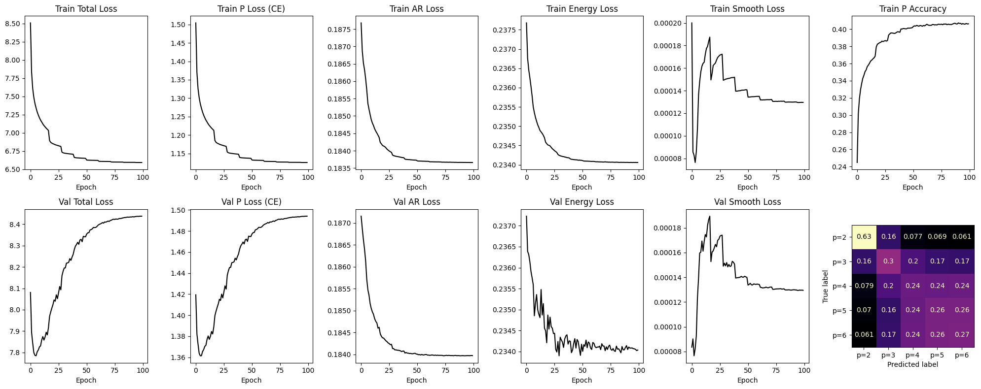
Train for 100 epochs with balanced loss weights. The training curve shows joint convergence of classification and regression objectives.

conf = {
    "lambda_ar": 5,
    "lambda_p": 5,
    "lambda_order": 0,
    "lambda_energy": 0.2,
    "lambda_smooth": 5,
}

model, history = do_bench_on_config(conf)
plot_history(history, model=model, val_loader=val_loader, device=device)

Training: 100%|██████████| 100/100 [14:56<00:00,  8.96s/it, p_acc=0.340, train=6.5934, val=8.4380]

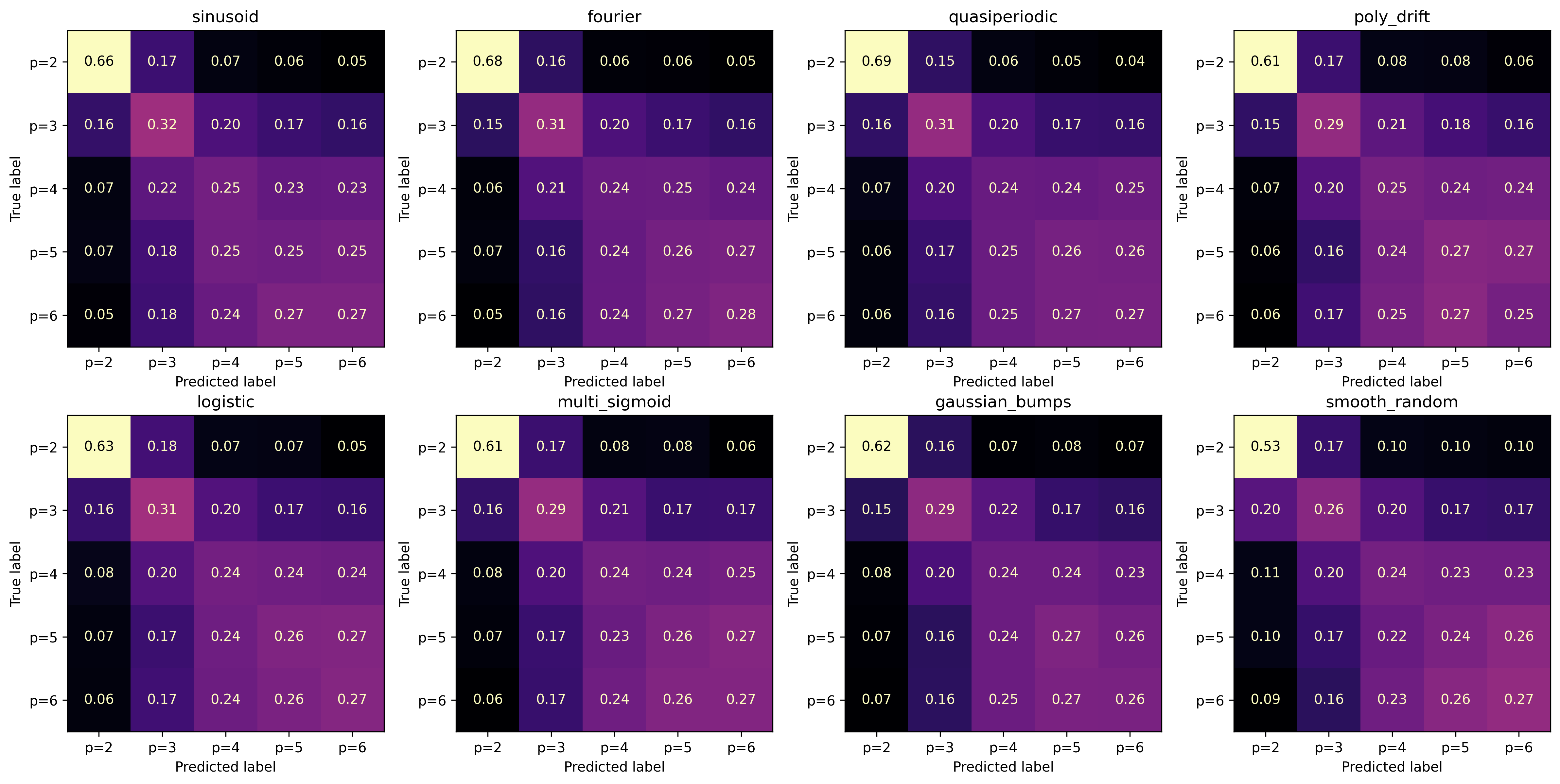
Evaluation: Order Classification

Confusion matrices show how well the model distinguishes AR orders within each family. Diagonal dominance indicates correct classification; off-diagonal mass reveals systematic over/under-estimation of \(p\).

# Get predictions on full validation set
model.eval()
all_p_pred = []
all_p_true = []

with torch.no_grad():
    for x_batch, p_batch in tqdm(val_loader, desc="Getting predictions"):
        x_batch = x_batch.to(device)
        _, _, p_hard, _ = model(x_batch)
        all_p_pred.extend(p_hard.cpu().numpy())
        all_p_true.extend(p_batch.cpu().numpy())

all_p_pred = np.array(all_p_pred)
all_p_true = np.array(all_p_true)

Getting predictions: 100%|██████████| 782/782 [00:00<00:00, 795.68it/s]

# Plot confusion matrix for each signal family
n_families = len(class_names)
nrows, ncols = 2, 4
fig, axes = plt.subplots(nrows, ncols, figsize=(4 * ncols, 4 * nrows), dpi=300)
axes_flat = axes.flatten()

p_min, p_max = 2, 6
n_classes = p_max - p_min + 1

family_results = {}

for i, family_name in enumerate(class_names):
    mask = class_id_val == i
    p_true_family = all_p_true[mask]
    p_pred_family = all_p_pred[mask]
    
    # Compute normalized confusion matrix
    cm = confusion_matrix(p_true_family, p_pred_family, labels=range(n_classes))
    cm_norm = cm / cm.sum(axis=1, keepdims=True)
    
    # Store accuracy for this family
    family_results[family_name] = {
        'accuracy': np.mean(p_true_family == p_pred_family),
        'n_samples': len(p_true_family)
    }
    
    # Plot
    disp = ConfusionMatrixDisplay(cm_norm, display_labels=[f'p={j+p_min}' for j in range(n_classes)])
    disp.plot(ax=axes_flat[i], cmap='magma', colorbar=False, values_format='.2f')
    axes_flat[i].set_title(f'{family_name}')

# Hide unused subplots
for j in range(n_families, nrows * ncols):
    axes_flat[j].set_visible(False)

plt.tight_layout()
plt.show()

Benchmark: Coefficient Recovery

Metrics per family:

• coeff_mse: Mean squared error of \(\hat{a}(t)\) vs true \(a(t)\)

• signal_mse: One-step prediction error using estimated coefficients

• p_acc: Classification accuracy for each order

family_bench_results = {}

for i, family_name in enumerate(class_names):
    mask = class_id_val == i
    X_family = X_val[mask].cpu()  # Move to CPU for bench_loop
    coef_family = coef_val[mask][:, :, :6]  # Slice to max_ar_order=6
    p_family = p_val[mask].cpu()
    
    results = bench_loop(model, X_family, coef_family, p_family, device)
    family_bench_results[family_name] = results

# Display as DataFrame
family_bench_df = pd.DataFrame(family_bench_results).T
family_df = family_bench_df.rename(columns={
    'coeff_mse': 'coeff mse',
    'signal_mse': 'signal mse',
    'p_mae': 'delta p',
    'p_mape': 'delta p / p',
    'p2_acc': 'p=2',
    'p3_acc': 'p=3',
    'p4_acc': 'p=4',
    'p5_acc': 'p=5',
    'p6_acc': 'p=6',
    'p_acc': 'P Avg.',
})
family_bench_df

	coeff_mse	signal_mse	p_mae	p_mape	p2_acc	p3_acc	p4_acc	p5_acc	p6_acc	p_acc
sinusoid	0.003924	0.183046	1.085483	0.290002	0.661209	0.326721	0.241122	0.251023	0.267625	0.351111
fourier	0.004272	0.184083	1.069846	0.284058	0.679984	0.316788	0.244737	0.274840	0.280372	0.358101
quasiperiodic	0.004035	0.182153	1.063116	0.281938	0.684039	0.310689	0.247123	0.272243	0.277012	0.356821
poly_drift	0.004315	0.183816	1.109580	0.302322	0.618354	0.300617	0.248848	0.262569	0.266481	0.340402
logistic	0.003673	0.183003	1.106807	0.300061	0.629938	0.296878	0.240559	0.260685	0.267918	0.339890
multi_sigmoid	0.003155	0.182505	1.132916	0.309419	0.607890	0.296363	0.244748	0.260765	0.269086	0.336374
gaussian_bumps	0.003542	0.183888	1.123097	0.302140	0.624358	0.305849	0.248492	0.266004	0.264642	0.340380
smooth_random	0.007759	0.189260	1.221906	0.343524	0.523409	0.258195	0.228875	0.251690	0.265594	0.305647

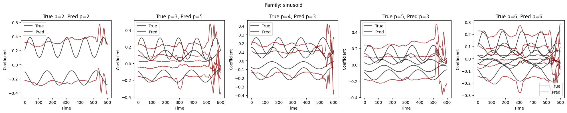
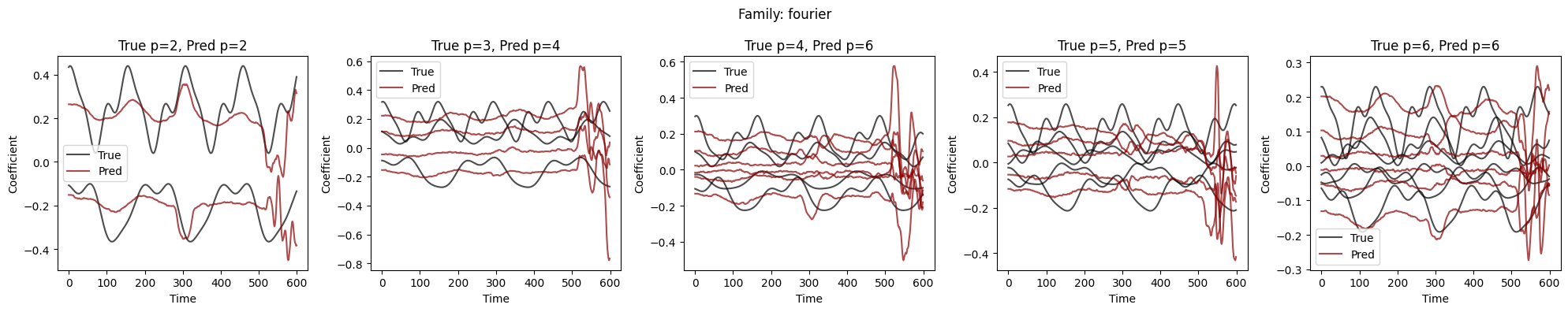
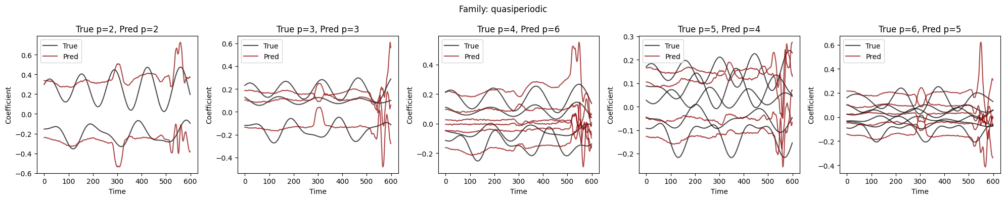
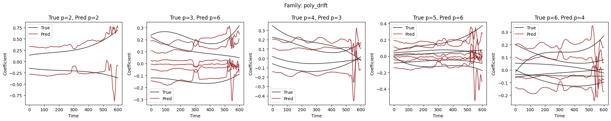
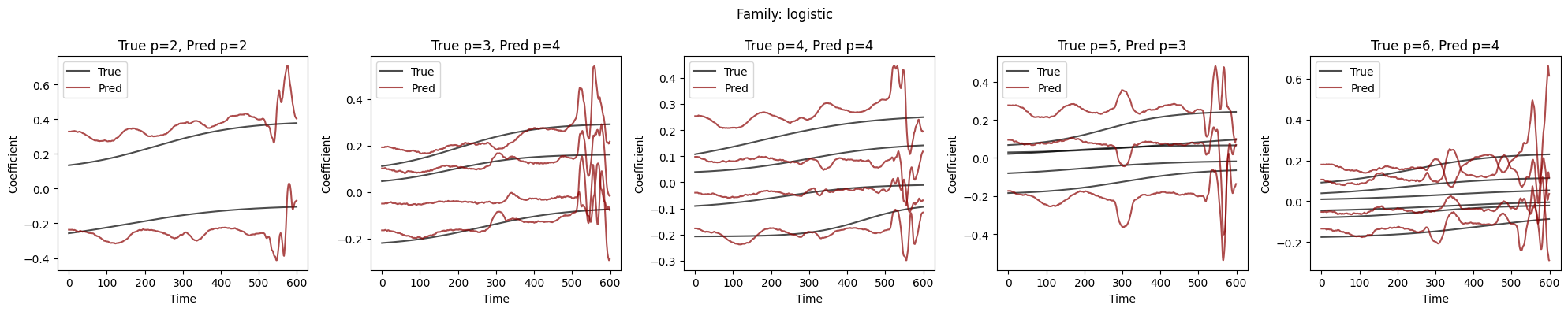
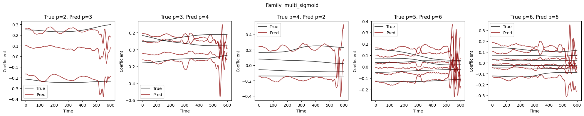
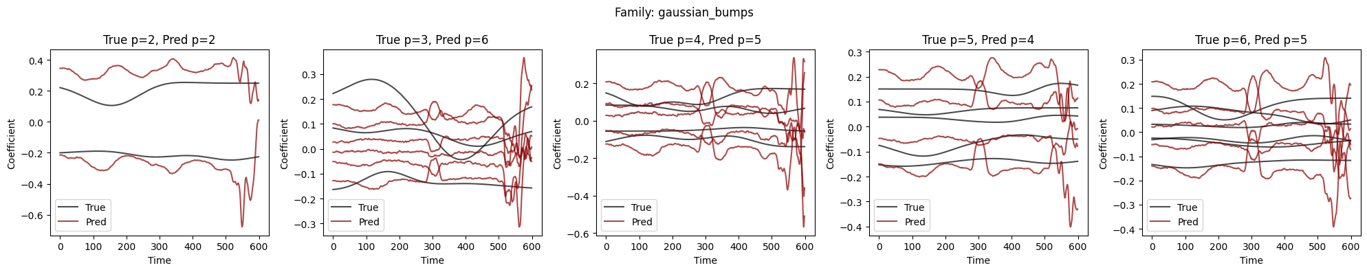
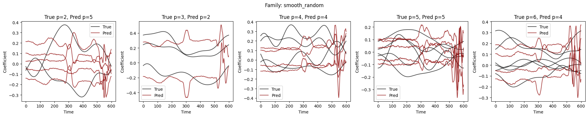
Visualize Coefficient Predictions

Overlay of predicted \(\hat{a}_k(t)\) (dashed) and true \(a_k(t)\) (solid) for representative samples. Good fits track the ground-truth dynamics; discrepancies highlight challenging regimes.

# Plot coefficient predictions for each signal family
for i, family_name in enumerate(class_names):
    mask = class_id_val == i
    X_family = X_val[mask].cpu()  
    coef_family = coef_val[mask][:, :, :6]
    p_family = p_val[mask].cpu()
    
    plot_coefficients_by_p(model, X_family, coef_family, p_family, device, 
                           p_max=6, p_min=2, title=f"Family: {family_name}")